Page 37 - rcf_152

37

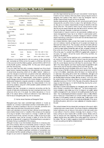
TABLE 2
Differencial and Difference Relationships among Six Basic Measurements
Six Basic Measurements and Their Classifications
Conventional Proposed Possible
Classification of
Wealth Momentum Force
Accounts by:
Measurements Measurements Measurements
Types of Wealth

(Assets, Liabilities) Wealth W
Reasons for Wealth
Change
Income ∆W Momentum Ẇ
(Revenues, Expen-
ses)
Reasons for Income or
Momentum Change
(Actions Resulting from Action ∆2W Impulse ∆Ẇ Force Ẅ
∆ Ẇ and the income ∆W are k
Impulses Created by
dollar/yr and k dollars, respectively, for the first year. Then compare this with
Forces)
a second project whose momentum starts at zero, increases uniformly to
Relationships among the Six Basic Measurements $1/yr at the end of the first year, and stays at that level from that point on.
2
Wealth: Income: Momentum: W(t+1) - W(t) = ∆W(t) = ∫t +1 Ẇ(r)dr (This is the case if a constant force Ẅ=$1/yr is applied with a duration of
Momentum: Impulse: Force: Ẇ(t+1) - Ẇ(t) = ∆Ẇ(t) = ∫t +1 Ẅ(r) one year.) The impulse ∆ Ẇ and the income ∆W are $1/yr and $0.5, res-
pectively, for the first year.
Income: Action: Impulse: ∆W(t+1) - ∆W(t) = ∆ 2 W(t) = ∫t +1 ∆Ẇ(r)dr
If K≥1, both a current-income maximizer and a current-impulse maximizer
differences in accounting standards in the two systems). will choose the first project, and if K≤0.5, both will chose the second project;
first while if 0.5<k<1, the current-income maximizer will choose the first project
while the current impulse maximizer will chose the second project. Who is
right in the choice depends upon how long the project is expected to earn
income at the rate that has been achieved at the end of the first year.
Suppose that both projects terminate at the end of year n. Then, the lifeti-
mes of incomes of the first and the second projects are kn dollars and 0.5+
(n-1)(or n-0.5) dollars, respectively. (Since the issue is on income and not
on cash flows, discounting will not enter into consideration, although it will
be briefly discussed later.) Hence, the current-income maximizer who choo-
ses the first project achieves a better life-time income if 1>k>1-0.5/n, while
the current-impulse maximizer who chooses the second project achieves a
better life-time income if 0.5<k<1-0.5/n. The ratio of the widths of the second
range over the first range is n-1(= [0.5-0.5/n]/[0.5/n]), favoring the current-
impulse maximizer for any n>2.
This issue of income versus impulses as managerial goals is related to the
choice of what is considered to be “status quo”. The income-based perfor-
mance evaluation views status quo to be no change in net wealth, giving
credit to management for any increase in net wealth generated by the ope-
ration. The impulse-based performance evaluation takes a totally different
notion of status quo. It views status quo to mean constant momenta, namely
the state of a firm earning income at a constant rate. Credit is given to the
management only for any increase in net momenta attributable to the opera-
tion during the period, and not to a mere realization of momenta created in
the past.

This contrast between the two viewpoints is analogous to the ways in which
moving bodies were viewed physics. Once it was commonly understood that
bodies could move only as long as a force acted on them and would come
to rest without it. Now it is common knowledge that in absence of force,
bodies continue to move linearly with a constant velocity. Bodies come to
rest not because the force supporting the move disappeared but on the
contrary because there was another force acting against the movement of
the bodies. This law of inertia suggests an important consideration in mo-
mentum accounting which will be considered next.

…………………………………………”